How to add maps to OpendTect?
Introduction
This post is associated with a couple of Jupyter notebook available on GitHub.
OpendTect is a great piece of software that allows you to load, process and interpret seismic data. In OpendTect, 2D lines and 3D volumes are displayed in a nice 3D environment that is easy to manipulate. Horizons, either 2D (lines) or 3D (surfaces) can be added to the 3D view alongside the seismic data.
In fact, any grid, not just seismic horizons, can be loaded in the OpendTect environment. This makes it ideal for displaying data from gravity and magnetic surveys. As a potential-field specialist, I am then able to compare directly the position of gravity and magnetic anomalies with the features that I see on seismic data.
While loading grids in OpendTect could be a tutorial on its own, in this post I will actually add one more difficulty by explaining how to load pictures, typically geological maps, to the 3D view. The solution I am proposing allows you to retain the original colours of the map (or at least most of them).
A map is typically created in a program like ArcGIS or QGIS and exported as an RGB coloured image, therefore containing 3 channels or bands (red, green and blue). The problem is that OpendTect cannot handle this type of image, it deals only with basic one-band grids. When they are rendered by OpendTect, one-band grids may appear in colours because the data are colour-coded (or mapped) to a list of colours, a colormap. Colormaps therefore help us to visualise the various intensities of the quantity contained in the grid. Note that we could also display a one-band grid with a grayscale, demonstrating it carries only intensity information.
So the trick to display RGB images in OpendTect is to merge the three bands into one, trying in the process not to lose too much information about the colours. This process is called colour quantization, or colour-depth reduction, and consists in finding for each colour in an image its closest match in a limited set of (predefined or not) colours.
The result is also called an indexed colour image because the colour information is stored in a separate file called a palette. The one-band grid therefore contains indices (or positions) representing a colour in the palette.
There are many methods and algorithms to achieve this result and the one I am proposing is specially targeting geological maps. These maps already contain a relatively small number of different colours: they represent the various types of rocks in an area, and, unless your area is particularly complex, there should be fewer than a hundred types (or ages, or whatever has been mapped). So the quantization should work pretty well in this case.
Method
To summarise what needs to be done to get a coloured map into OpendTect, here is a breakdown of the method:
- Prepare the RGB image of the map.
- Convert the image from RGB to indexed colour using color quantization.
- Crop and resample the image to fit the OpendTect survey area.
- Import into OpendTect.
The first step could involve extracting a picture from a PDF file, or exporting an image from a GIS application. Additionally, the map might also need to be georeferenced and/or projected in the same coordinate system as the seismic data. We will assume in the following that this stage has already been completed.
Example: the Kevitsa Deposit, northern Finland
In order to describe the method more efficiently, I am using an example based on some data that have recently been made freely available thanks to the Frank Arnott award. It is a complete geophysical dataset that has been used for the exploration of the Kevitsa intrusion in Finland (Malehmir et al., 2012). It contains a 3D reflection seismic survey, potential-field survey data, wells, geological maps and cross-sections.
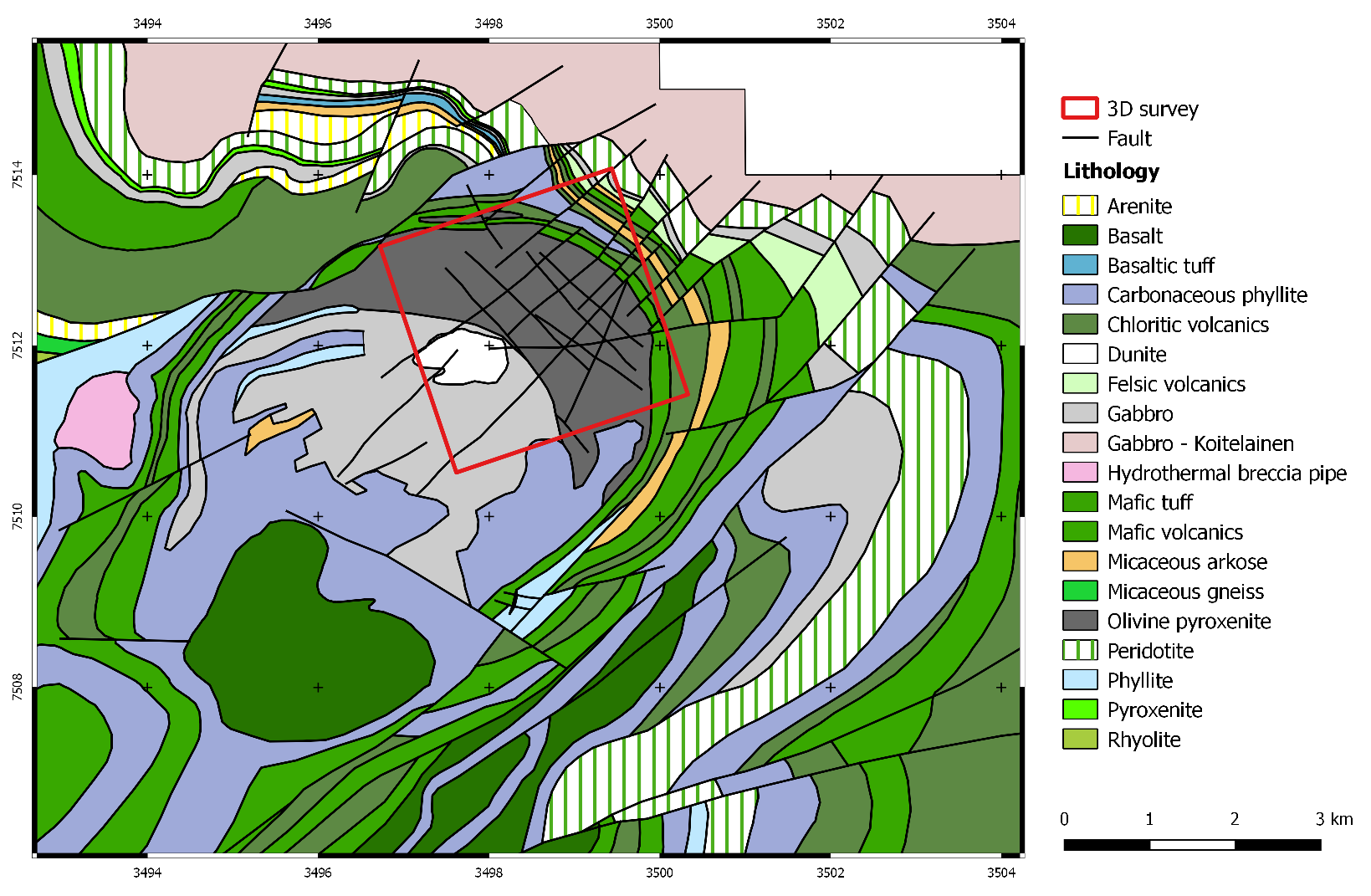
The mafic-ultramafic intrusion has an elliptical shape in map view and the 3D seismic survey is located on its north-east side (Figure 1). The intrusion is surrounded by sedimentary and volcanic rocks that are both folded and faulted. The seismic data were used to image the contact between the intrusion and the adjacent units, as well as the geometry of the intrusion at depth (Koivisto et al., 2015).
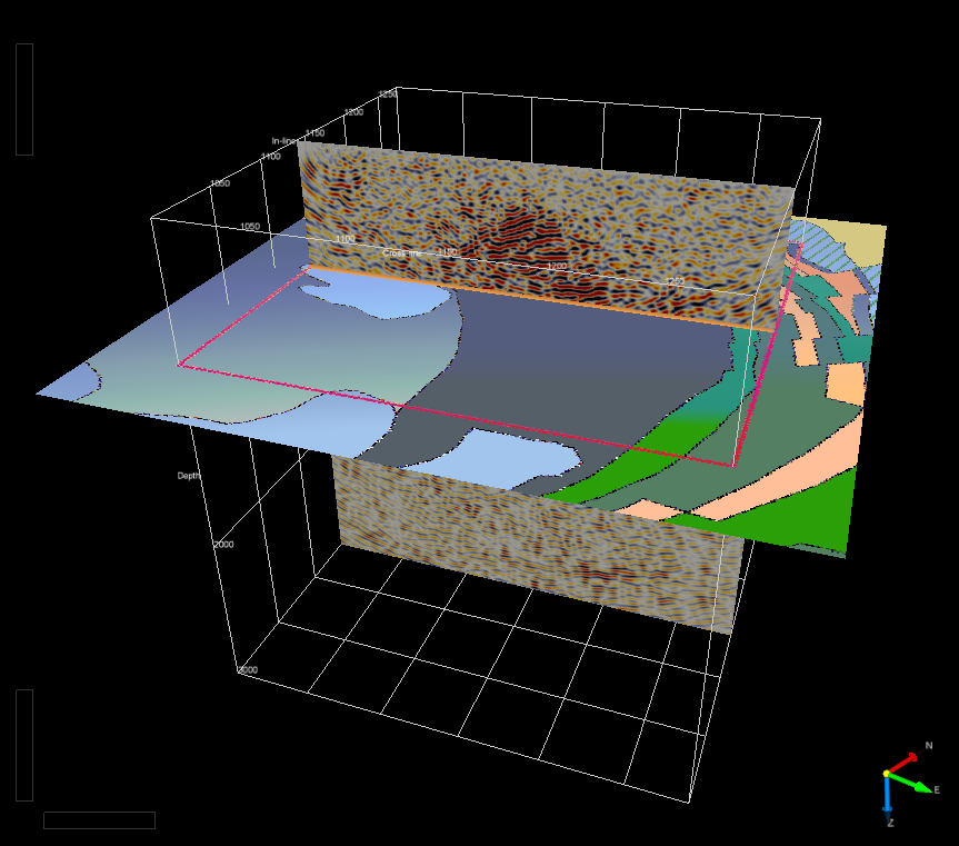
So the purpose of this exercise is to have an image of the geological map rendered together with the seismic data in a 3D environment. The first stage of this process is to extract a portion of this map centred on the 3D survey. The legend, the scale and other annotations are superfluous for this purpose, as only the geological information is required (Figure 2).
Georeferencing
It is essential for the final step of the method (interpolation onto the OpendTect survey grid) to have the geographic coordinates of the image, i.e. its location and its extent. This information will be contained in a world file that is automatically created by QGIS or by ArcGIS when the map is exported to a PNG file. Look for a small .pgw text file with the same name as the PNG file. These two files (the .png and the .pgw) always need to sit together on your drive.
Color Quantization
This is the conversion of our RGB image to a one-channel image using a specific set of colours.
Palette
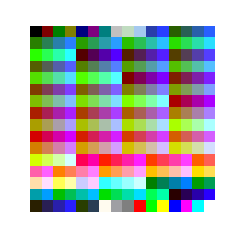
I am using a fixed palette of 256 colours. Fixing the colours can potentially degrade the performance of the quantization process, but this is essential for OpendTect to render our images consistently. It is also much simpler, as the alternative would be to have a different palette for each image, which is impractical.
This palette is the classic Windows palette (Figure 3). It contains a number of shades of red, green and blue-ish colours, and also the typical set of basic colours that are found in lots of Windows programs. A text file with the RGB colours of the palette can be found here.
Pairwise distance
The quantization can be simply performed with a function of the scikit-learn Python library. Its metrics sub-module contains functions to compute distances between objects. We need a function that can tell us the colour in the palette that is the closest to the colour of each pixel in our RGB image.
This function is called pairwise_distances_argmin and using it for color quantization is straightforward. Here is the gist of the method in Python code:
from sklearn.metrics import pairwise_distances_argmin

indices = pairwise_distances_argmin(flat_array, win256)
indexedImage = indices.reshape((nrows, ncols))
Here, win256 is a 3-column array containing the 256 colours of the Windows palette. It is compared with flat_array, which is a reshaped version of our initial RGB image. The result is a list of indices pointing at the colours in our palette. To get our final grid, we finally need to reshape the result back to a rectangular array that has the same dimensions as the initial image.
A more complete version of the code is available in this Jupyter notebook.
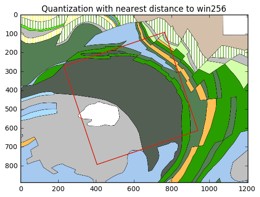
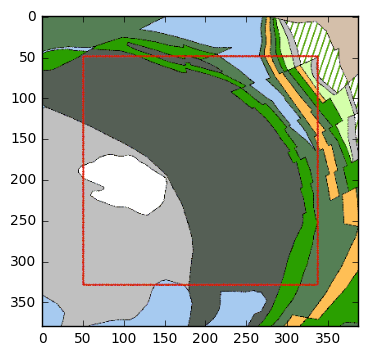
The result is our quantization method is quite good and looks almost identical to the original (Figure 4). Of course, in order to display it properly we also need to have the Windows 8-bit palette loaded as a colormap in matplotlib (see the notebook for the details).
Cropping and Resampling
Having the RGB image converted to a one-band grid is only one part of the process of importing the map into OpendTect. The other non-trivial bit is to make sure the position and sampling of the grid correspond exactly with the grid that defines the “Survey” in OpendTect. As the OpendTect documentation puts it: “Projects are organized in Surveys - geographic areas with a defined grid that links X,Y co-ordinates to inline, crossline positions. 3D seismic volumes must lie within the defined survey boundaries.”
From this point onwards, there are two possibilities: either you have an actual 3D seismic volume loaded in your project, or you have only 2D seismic lines. In the first scenario, the 3D volume dictates the geometry of the OpendTect survey. In the latter case, you are actually free to define the survey grid, since “2D lines and wells are allowed to stick outside the survey box”.
Survey definition
So for the simple 2D case, my advice is generally to use a grid that defines a rectangle area that encompasses most or all the 2D lines. The grid needs to be in the same projected coordinate system as the seismic. The common scenario is that a gravity or a magnetic survey is available in the area, so this is the grid that should be used for the OpendTect survey.
In contrast, 3D seismic surveys come in all sorts of shape and orientation so a mismatch is likely to occur between the survey grid and the map we want to import. Cropping and resampling the map are therefore necessary.
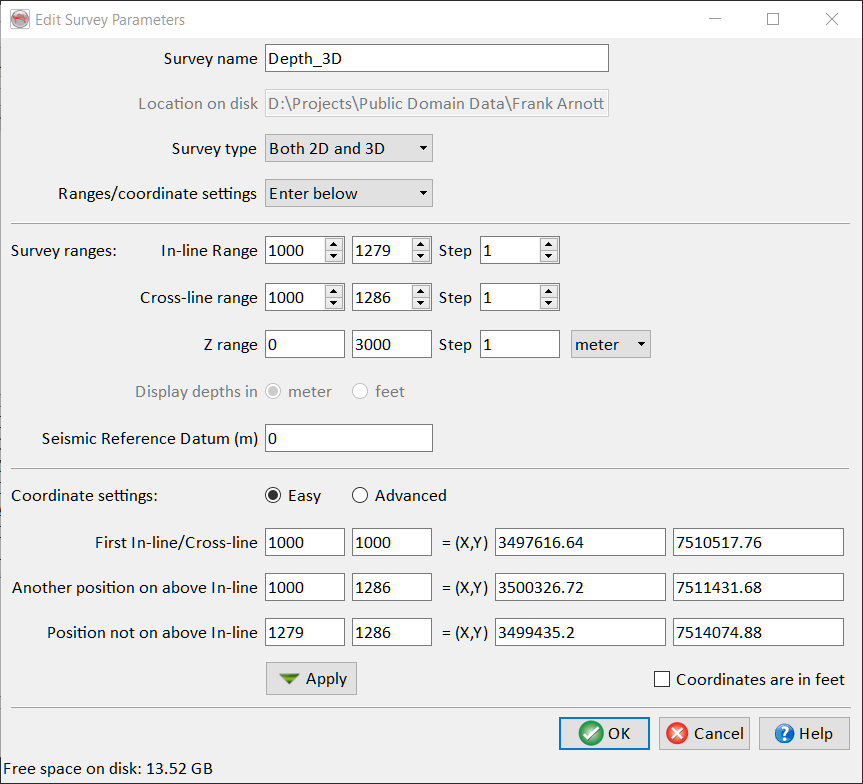
In the Kevitsa example, the outline of the seismic cube makes an angle of about 20 degrees with the north. In OpendTect, the Survey grid is created by scanning the coordinates of the traces in the SEGY file. The result shows that the grid comprises 280 in-lines and 287 cross-lines (Figure 5).
Interpolation
Cropping and resampling are performed in one pass by interpolation onto the grid that defines the location of the OpendTect survey. The SciPy interpolate module contains the functions we need for this purpose.
The important task before running the interpolation is to create two sets of coordinates: one for the grid of our image and one for the target grid, i.e. the seismic survey.
As stated earlier, the coordinates of our input image were exported by QGIS when we created the image of the map. In Python, we load the image and its attached geographic metadata with the rasterio module (see Jupyter notebook). We could also directly open the .pgw file in a text editor and read the cell size and location of the upper left pixel.
Keep in mind when reading coordinates of raster images that these numbers could correspond to either the centre or the corner of the pixel. There are two conventions for registering images (gridline- and pixel-based) and both are equally used. For example, rasterio would give you the position of the corner of the upper-left pixel, while the world file gives you its centre.
In any case, constructing a grid of coordinates with Numpy is easy thanks to the meshgrid function:
# 1-D arrays of coordinates
x = np.linspace(xmin,xmax,num=ncols,endpoint=False)
y = np.linspace(ymin,ymax,num=nrows,endpoint=False)
# 2-D arrays of coordinates
X,Y = np.meshgrid(x,y)
Y = np.flipud(Y)
The X and Y arrays give the coordinates (X[i,j], Y[i,j]) of each pixel (i,j) in the image. Flipping the Y array upside-down is necessary because indices are counted from the top down, while the y-coordinate (northing) increases northward.
The arrays for the target grid are created slightly differently. First we create arrays of in-line and cross-line indices (trace numbers) as defined in OpendTect. Then the coordinates are calculated using the formulas of the affine transformation that are provided in Survey Setup > Coordinate settings (advanced panel, Figure 6).
The coordinates of the target grid are therefore given by:
inline_limits = np.arange(1000,1280,1)
xline_limits = np.arange(1000,1287,1)
inline,xline = np.meshgrid(inline_limits,xline_limits,indexing='ij')
# indexing starts from bottom-left corner
inline = np.flipud(inline)
# Now we can compute the coordinates
Xi = 3491336.248 - 3.19541219*inline + 9.4758042*xline
Yi = 7497848.4 + 9.47383513*inline + 3.19552448*xline
The last stage consists in combining all these elements together by first creating the interpolation function with the first grid and then running it onto the second grid.
points = np.column_stack((X.flatten(),Y.flatten()))
values = indexedImage.flatten()
interp = interpolate.NearestNDInterpolator(points,values)
newImage = interp((Xi,Yi))
It is important to use the nearest-neighbour interpolator here because we need to preserve the values of our indexed colours. Otherwise, the colours of our image could change in an unexpected way!
The result looks great and shows the map rotated in the frame of the 3D seismic survey (Figure 7). Note that the image is a bit bigger than the outline of the 3D because I have extended the target grid by 50 pixels on all sides (see the Jupyter notebook for the code to achieve that).
Importing the grid into OpendTect
The final step is to actually import the grid of our indexed-colour rotated image into OpendTect. The grid will be imported as a 3D horizon geometry and the colour information will be imported as an attribute. Both operations can be performed at the same time. But first, our grid needs to be saved in a format that OpendTect can read, the simplest one being an ASCII column format.
Since we have deliberately created the new image to match the grid of the survey data, the inline and crossline trace numbers can be used instead of the X and Y coordinates. The code to make the ASCII text file is available in the Jupyter notebook.
Importing the file in OpendTect is easy:
Go to Survey > Import > Horizon > ASCII > Geometry 3D…
Select the newly created .xyz file.
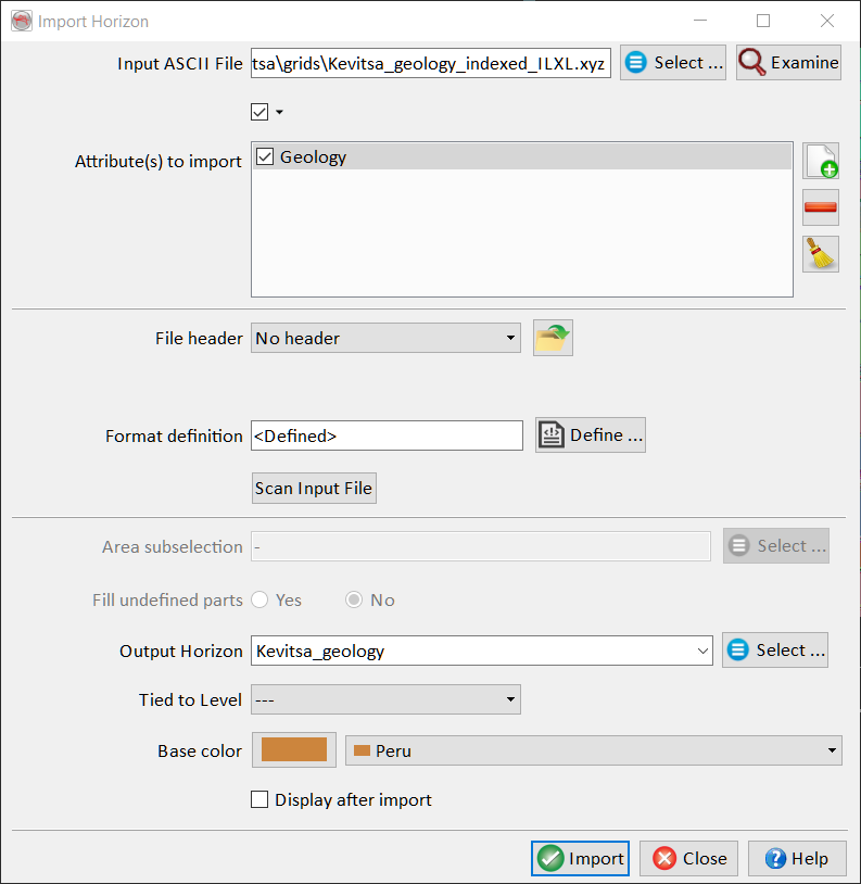
Add the colour indices (the pixel values) as an attribute called “Geology”.
Define the format by clicking “Define…”.
Select “Inl Crl” instead of “X Y” in the dropdown menu.
The rest of the format definition should automatically be correct since we have added a Z column in the third position. Define the name of the output horizon and the Import Horizon window should look like Figure 8.
Displaying the map in OpendTect
Our new 3D horizon can now be added to the display by clicking on “3D Horizon” in the scene Tree, then click “Add…”. Select the horizon in the list and click OK. You should see a flat plane at depth = 0 with a single bright colour. This is because OpendTect displays the Z-values of the horizon by default. To show the actual colours of the geological map, right-click on “Z value” in the Tree, then “Select Attribute” and “Horizon Data (1)…”. Select “Geology” in the list.
Loading the correct colormap
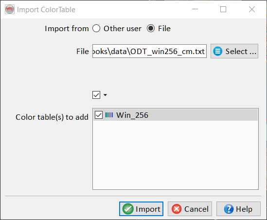
The map should now be displayed in the 3D scene in the right location related to the seismic data. However, the colours are likely to be completely wrong! This is because there is one last piece missing: the Windows 8-bit palette we used for the quantization. It needs to be imported as a new “ColorTable” (Figure 9). The file is available here.
To import the correct palette, follow these steps:
go to Survey > Import > ColorTable…
Select Import from: File.
Browse to the location of the text file that contains the color table
Select “win_256” in the list of “Color table(s) to add”
The final task is to assign the new Color Table to the “Geology” attribute. Select the attribute in the scene tree, then choose “Win_256” in the dropdown list of ColorTables. Make sure the range of the color scale goes from 0 to 255.
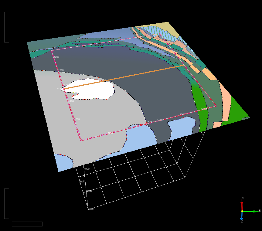
Et voila! The map is not displayed in all its glory together with the seismic data of the 3D survey (Figure 10 and Figure 11).
Conclusion
While not completely straightforward, importing geological maps in OpendTect is possible! ;-)
Acknowledgements
The geological map and the 3D seismic survey were kindly made available through the Frank Arnott Award by First Quantum Minerals Ltd. The content of the dataset is re-used here with permission.
References
Koivisto, E., Malehmir, A., Hellqvist, N., Voipio, T., Wijns, C., 2015. Building a 3D model of lithological contacts and near-mine structures in the Kevitsa mining and exploration site, Northern Finland: Constraints from 2D and 3D reflection seismic data. Geophysical Prospecting 63, 754–773. doi:10.1111/1365-2478.12252
Malehmir, A., Juhlin, C., Wijns, C., Urosevic, M., Valasti, P., Koivisto, E., 2012. 3D reflection seismic imaging for open-pit mine planning and deep exploration in the Kevitsa Ni-Cu-PGE deposit, northern Finland. Geophysics 77, WC95-WC108. doi:10.1190/geo2011-0468.1
