Three notebooks to jump start a data science project
Introduction
I was in Paris last week for the 2017 Subsurface Hackathon. It was superbly organised by Agile Scientific and Total. Together, they managed to draw a large (about 60 persons) and diverse crowd to participate to the challenge of producing some working and usable software in only two days. The event took place over the weekend just before the EAGE conference, so you could tell people were highly motivated to come and share the experience.
I was with Martin Bentley in a small team called Water Underground. While Martin was actually sitting in Port Elizabeth in South Africa, I was in La Defense in Total’s brand new offices. Our idea was to mine some groundwater data from the Geological Survey of the Netherlands and use the measurements to predict the evolution of water depth and composition both in space and time. Unfortunately, we did not manage to complete the project. As any data scientist would tell you, the first (and somewhat less rewarding) steps of any data science project can take a lot of time, generally more than expected…
The Data Science Process
There are loads of resources out there that would detail the various stages of a data science project. At the end of the day, any research project would probably follow this sort of process:
- data acquisition
- data preparation, cleaning and transformation
- data exploration
- modelling and predictive analysis
- interpretation of the results
- communication of the results
Having spent a couple of days on the first three steps of this process, I decided I could share the code and the notebooks I wrote because some of this material is rather generic and can easily be re-used for other projects. There are a few tips and tricks about how to use pandas and Python notebooks for data analysis, so hopefully those can be useful to anyone interested in starting this sort of project.
The notebooks are available in a GitHub repository.
Groundwater data in the Netherlands
The dataset we used (and barely started to explore…) is a set of groundwater wells in the Netherlands. Groundwater levels have been measured in some locations on a monthly basis since the 1950’s. So it’s a truly 4D dataset: you can either look at single wells in isolation for time-series analysis, or construct a surface of the water table at a given time by interpolating between points.
To come back to the initial steps of the data science project, here are brief descriptions of what can be found in the notebooks for each step.
Data acquisition and cleaning

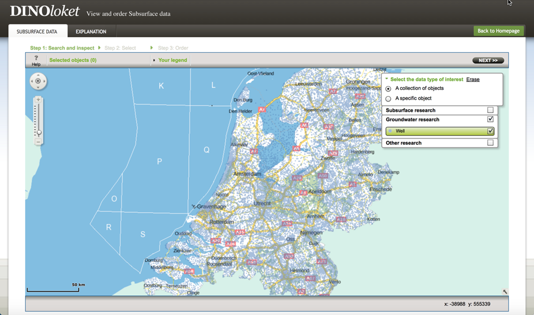
The data files were selected manually and downloaded from the DINOloket website. The files are provided either as CSV files, or as space-delimited text files. Large headers of variable dimensions make the import into pandas unnecessarily difficult. Additionally, the headers are in Dutch. Thankfully, Martin managed to translate the text and found the logic in the headers. This is all described in the METADATA file on his own GitHub project.
Some basic exploratory analysis is carried out at the end of the notebook.
The notebook for this step is here.
Data transformation
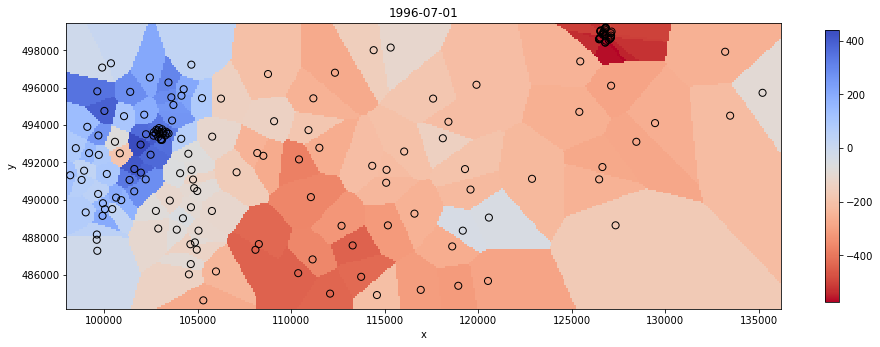
That’s where it starts to be interesting. In this second notebook, I demonstrate how to create a surface from well data by using the Scipy function griddata. Gridding all the points turns out to be meaningless because the measurements do not cover the same period for all the wells.
Resampling the data in time becomes therefore essential. This is where the strength of pandas is obvious as this step can be done with only one line of code.
Once the depth measurements have been resampled to follow a constant frequency at all the wells, it becomes very easy to make a selection for a given month and grid up the result. Here is an example:

Data exploration
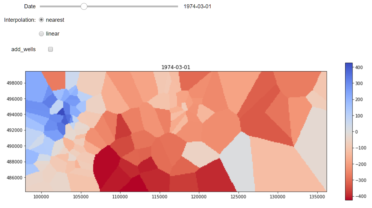
The third and final notebook provides a convenient way to explore this large dataset. Using the ipywidgets library, I create two interactive plots, one for the surface and one for the time series. A slider can be used to select the date and a dropdown menu gives access to the list of wells.

Conclusion
The hackathon was a great opportunity to meet a lot of people interested in open source software, machine learning and geoscience. I think the time and efforts that went into our project, even it was not completed, should also benefit the wider community. So here is my contribution. If you ever pick up this project where we left it and make some more progress, please get in touch!