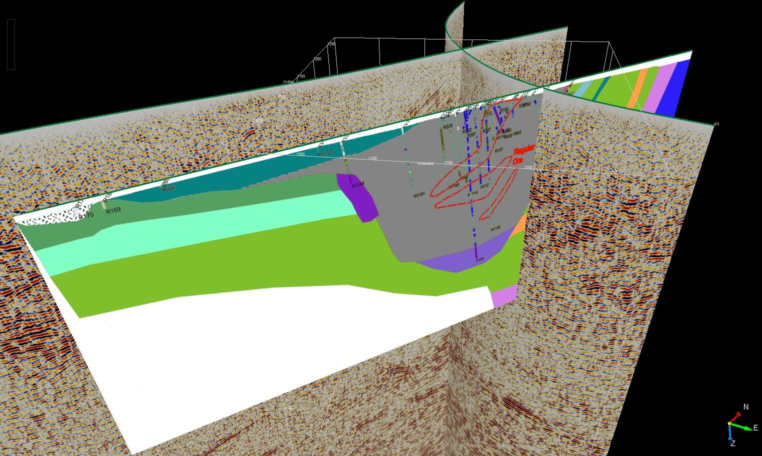
How to add cross-sections to OpendTect?
Introduction
This post is associated with a Jupyter notebook available on GitHub.
In a previous post, I explained how to add colour maps to the 3D environment of OpendTect. The method is simply to convert the RGB image of the map into an indexed colour image. The resulting grid can be loaded as any other horizon and the colours are provided by a fixed palette.
In this post, I will show how to apply the same method to insert images of cross-sections to OpendTect. This is in essence a conversion of an image into seismic data.
Method
The basic steps of the method can be described as follows:
Prepare the RGB image of the cross-section.
Resize and resample the image to fit the appropriate dimensions of the section.
Convert the image from RGB to indexed colour using colour quantization
Import the result into OpendTect as seismic data.
While this seems straightforward, there can be several issues on the way. Problems are mostly related to the proper positioning of the cross-section in space.
One relatively important point to note is that resampling should ideally happen before colour quantization. This is because resampling might modify the colour index, which is an integer. Of course, one way to avoid this problem is to use nearest-neighbour interpolation during resampling (see the previous post).
Example: the Kevitsa Deposit, northern Finland
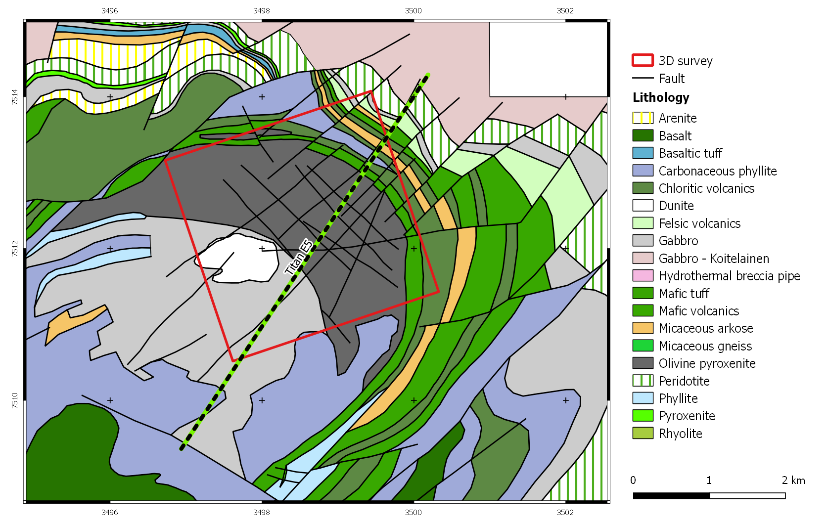
In order to describe the method more efficiently, I am using an example based on data that have recently been made freely available thanks to the Frank Arnott award. It is a complete geophysical dataset that has been used for the exploration of the Kevitsa intrusion in Finland (Malehmir et al., 2012). It contains a 3D reflection seismic survey, potential-field survey data, wells, geological maps (Figure 1) and cross-sections.
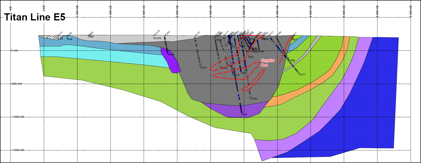
For this demonstration, I am using a cross-section called Titan Line E5 that runs across the Kevitsa mafic-ultramafic intrusion (Figure 1). The section was produced by interpretation and inversion of magnetotelluric (MT) and electromagnetic measurements that were collected by Quantec Geoscience Ltd during a survey in 2008. The interpretation, performed by First Quantum Minerals Ltd, shows the shape of the main olivine pyroxenite intrusion, the presence of smaller dunite bodies, and the surrounding sedimentary and volcanic rocks (Figure 2).
Resizing and Resampling
One of the difficulties with importing images of cross-sections is the presence of annotations, text and other grids. It is therefore important to start the process with a clean image that has been stripped of those disturbing elements. When importing from a PDF file, a program like Inkscape can be very useful to extract only the essential information.
The cross-section is georeferenced (generally) by its start and end points, both in the horizontal and vertical dimensions. So a tight crop of the image to these reference points is the next step. Sometimes a gain in precision can be achieved by removing bits on the sides. For example, in my example of the Titan Line E5, I cropped the bottom of the image to a depth of 1500 m instead of trying to estimate the actual depth of the deepest point of the section.
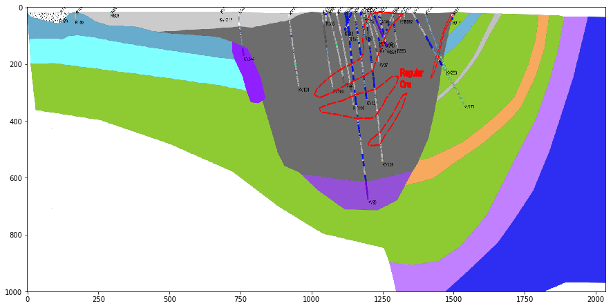
Once a good quality image of the section is obtained, it might be necessary to resample it to match the typical dimensions of a seismic line in the project you are working on. “Pixels” in seismic data are rarely square, i.e. the spaces between traces and samples in depth-converted data are not equal. In effect, the seismic “pixel” is stretched in the horizontal dimension. This ensures a good resolution in the vertical dimension, especially as most people would actually apply a large vertical exaggeration when doing any interpretative work. So to replicate this in our case, we need to oversample the image in the vertical dimension.
For the Titan line, I have increased the number of pixels in the Z dimension (the number of rows) from 704 to 1000 (Figure 3). Details about the Python implementation can be found in this Jupyter notebook.
Colour Quantisation
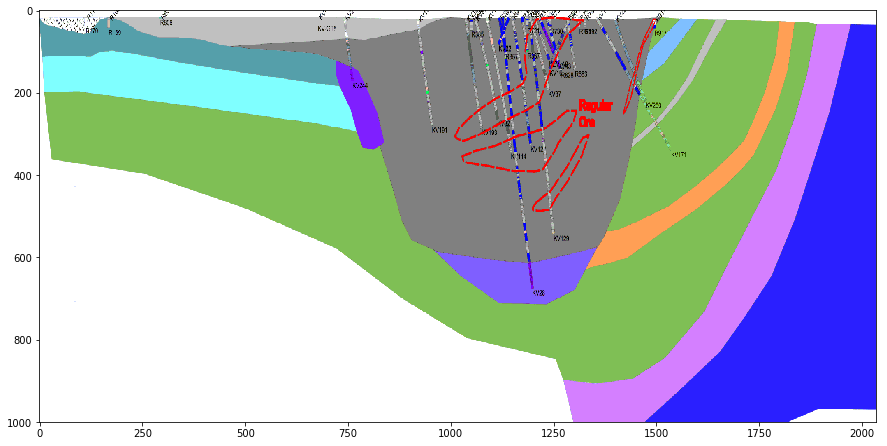
This stage in the process is very similar to what was done in the case of maps. I use scikit-learn and a pairwise distance function to match the colours in the image with one of 256 colours of a fixed palette (the 8-bit Windows palette).
Since the cross-section makes use of simple coloured patches, the quantised result looks almost identical to the original RGB picture (Figure 4). The advantage of course is that there is only one band instead of three.
Conversion to SEGY
The quantised image now needs to be converted to a format that OpendTect can understand. While the simplest solution might be to use a text file in an ASCII format (“Simple File” in OpendTect jargon), I am converting the section to the SEGY format as this makes the method more generic. This also gives me the opportunity to use the obspy library!
Referring to the final cells of the notebook, here is a breakdown of this stage:
Using the coordinates of the start and end points of the line, a bit of Python code is used to calculate the coordinates of each trace (each column in the image) by linearly interpolating between the two extremities.
The next step is to define some parameters like the coordinate scaling factor and the sample interval. The scaling factor makes it possible to store coordinates at centimetre-scale precision using only integers.
Optionally, a text header can be added to the file to keep some information about the data.
The final step is to write all this information to file.
Importing the section in OpendTect
While loading the resulting SEGY file into OpendTect should be straightforward and identical to importing “normal” seismic data, it is essential to also add the 8-bit palette of 256 colours that were used for the quantisation. I refer you to the end of the previous post for the instructions on how to do that.
Conclusion
Having the cross-section side-by-side with the reflection seismic data and the geological map in a 3D environment helps to appreciate the differences and similarities between these three types of information (Figure 5). The dataset could be completed to include wells, magnetic data, other cross-sections, etc. It would then become the ideal tool for exploration in this part of the world.
References
Koivisto, E., Malehmir, A., Hellqvist, N., Voipio, T., Wijns, C., 2015. Building a 3D model of lithological contacts and near-mine structures in the Kevitsa mining and exploration site, Northern Finland: Constraints from 2D and 3D reflection seismic data. Geophysical Prospecting 63, 754–773. doi:10.1111/1365-2478.12252
Malehmir, A., Juhlin, C., Wijns, C., Urosevic, M., Valasti, P., Koivisto, E., 2012. 3D reflection seismic imaging for open-pit mine planning and deep exploration in the Kevitsa Ni-Cu-PGE deposit, northern Finland. Geophysics 77, WC95-WC108. doi:10.1190/geo2011-0468.1
